In doing research on the Fourier Transform, I have had some interesting insights that I would like to share here.

Transform Definitions

Classical Definitions

The (classical) Continuous Time Fourier Transform (cCTFT) \({\cal F}_{\mathbb{R}}\) of a function \(f:\mathbb{R} \rightarrow \mathbb{R}\) is given by

\[{\cal X}_{\mathbb{R}}\{f\}(\omega) := \int_{-\infty}^{\infty} f(t) e^{-i \omega t} \; dt.\]

The (classical) Discrete Time Fourier Transform (cDTFT) \({\cal F}_{\mathbb{Z}}\) of a function \(f:\mathbb{Z} \rightarrow \mathbb{R}\) is usually given by

\[{\cal X}_{\mathbb{Z}}\{f\}(\omega) := \sum_{t=-\infty}^{\infty} f(t) e^{-i \omega t}.\]

Moving Towards a Unified Definition

The cDTFT definition feels and looks correct, since it looks exactly like the continuous time definition, but with the integral replaced by a sum. I would tend to agree, but I study time scales, which seeks to unify the continuous and discrete under one analytic framework. One issue I have with this definition is that the domain of both transforms is the same: \(\omega\) can be any real number. In reality, the cCTFT and cDTFT can both be thought of as being evaluated on the cusp between the unstable region and the stable region of the Laplace Transform and the Z-Transform, respectively. This means the domain of the cCTFT is \(\mathbb{R}\), as we already have, but the domain of the cDTFT should really be the unit circle. Let’s make this more explicit by defining the cDTFT in terms of the variable \(e^{i \omega}\), which is always on the unit circle.

\[{\cal X}_{\mathbb{Z}}\{f\}(e^{i \omega}) = \sum_{t=-\infty}^{\infty} f(t) \frac{1}{( e^{i \omega} )^t }.\]

Now, the exponential function in the denominator of the integrand above is looking like the delta exponential on the integers, but without the shift of plus one. Define the new variable \(\xi = (e^{i \omega} -1)/i\). Notice since \(e^{i \omega}\) is always on the unit circle, \(\xi\) is always on the unit circle shifted left by one, then rotated by \(-\pi/2\) radians (this is the same as saying \(\xi\) is on the unit circle shifted up by one unit) This leads to the same cDTFT in terms the new variable \(\xi\),

\[{\cal X}_{\mathbb{Z}}\{f\}(\xi) = \sum_{t=-\infty}^{\infty} f(t) \frac{1}{(1+i \xi)^{t}}.\]

Notice nothing has really changed from the orginal cDTFT definition. I have simply recontextualized the definition and made one change of variable (notice \(1+ i \xi = e^{i \omega}\), so the denominator has remained the same).

Now, for reasons that will be revealed later, I actually want to alter the definition of the cCTFT and cDTFT to arrive at the (unified) Continuous Time Fourier Transform (uCTFT) and (unified) Discrete Time Fourier Transform (uDTFT)

Unified Continuous Time Fourier Transform Definition

For the cCTFT, let \(\xi = \omega\) and define the uCTFT of \(f\), \({\cal F}_{\mathbb{R}}\), as

\[{\cal F}_{\mathbb{R}}\{f\}(\xi) := {\cal X}_{\mathbb{R}}\{f\}(\xi).\]

That is, the cCTFT and uCTFT are exactly the same, except I am renaming \(\omega\) as \(\xi\) (thrilling, I know).

Unified Discrete Time Fourier Transform Definition

For the cDTFT, let \(\xi = (e^{i \omega} - 1)/i\) and define the uDTFT of \(f\), \({\cal F}_{\mathbb{Z}}\), as

\[\begin{aligned} {\cal F}_{\mathbb{Z}}\{f\}(\xi) & := \frac{1}{1+i \xi} {\cal X}_{\mathbb{Z}}\{f\}(\xi) \\ & = \sum_{t=-\infty}^{\infty} f(t) \frac{1}{(1+i \xi)^{t+1}}. \end{aligned}\]

I have added in a forward shift to preserve operational properties.

Operational Properties

The differential operator of \(\mathbb{R}\) is the derivative. The differential operator I want to use on \(\mathbb{Z}\) is the forward difference \(\Delta f(t):= f(t+1)-f(t).\) There is a key property that uCTFT and uDTFT share with respect to their respective differential operators.

uCTFT of a Derivative

Using integration by parts and the fact that acceptable signals must go to zero as time approaches infinity in either direction gives us

\[\begin{aligned} {\cal F}_{\mathbb{R}}\{f'\}(\xi) & = \int_{-\infty}^{\infty} f'(t) e^{-i \xi t} \; dt. \\ & = f(t) e^{-i \xi t} \rvert_{-\infty}^{\infty} - \int_{-\infty}^{\infty} f(t) - i \xi e^{-i \xi t} \; dt \\ & = 0 + i \xi \int_{-\infty}^{\infty} f(t) e^{-i \xi t} \; dt \\ & = i \xi {\cal F}_{\mathbb{R}}\{f\}(\xi). \end{aligned}\]

uCTFT of a Forward Difference

Note that \(\begin{aligned} \frac{1}{1+i \xi} ({\cal F}_{\mathbb{Z}}\{\Delta f\}(\xi) - i \xi {\cal F}_{\mathbb{Z}}\{f\}(\xi)) &= \sum_{t=-\infty}^{\infty} \frac{(f(t+1) - f(t)) - i \xi f(t)}{(1+i \xi)^{t+2}} \\ & = \sum_{t=-\infty}^{\infty} \frac{f(t+1)-(1+i \xi) f(t)}{(1+i \xi)^{t+2}} \\ & = \sum_{t=-\infty}^{\infty} \frac{f(t+1)}{(1+i \xi)^{t+2}} - \frac{f(t)}{(1+i \xi)^{t+1}} \\ & = \sum_{t=-\infty}^{\infty} \frac{f(t+1)}{(1+i \xi)^{t+2}} - \sum_{t=-\infty}^{\infty} \frac{f(t)}{(1+i \xi)^{t+1}} \\ & = {\cal F}_{\mathbb{Z}}\{f\}(\xi) - {\cal F}_{\mathbb{Z}}\{f\}(\xi) \\ & = 0 \end{aligned}\)

Thus \({\cal F}_{\mathbb{Z}}\{\Delta f\}(\xi) = i \xi {\cal F}_{\mathbb{Z}}\{f\}(\xi).\) This matches how the unified transform interacted with the differential operator on \(\mathbb{R}\)

Okay, I have to be honest here that we didn’t need the extra \((1+i \xi)\) in the denominator for this to work out on \(\mathbb{Z}\). But, the shift forward is absolutely essential when trying to make this work on arbitrary time domains.

Domains

The uCTFT is defined on the real line. The uDTFT is defined on the unit circle shifted up by one, so it is tangent to the real axis and in the upper-half plane.

Let’s think about the time domain \(h \mathbb{Z} = \{...-3h, -2h, -h, 0 , h, 2h, 3h, ...\}.\) For \(s \in h \mathbb{Z}\), one can perform the change of variables \(t= s/h\) and perform a uDTFT. However, looking at the domain of this transformation in the orginal domain, we see the domain of the transform is the disc of radius \(1/h\) that is tangent to the real axis and in the upper-half plane. This lets us see a beautiful unity in our approach. As \(h \rightarrow 0\), the domain of the Fourier transform becomes a bigger and bigger circle, so big that the bottom part of the circle becomes almost a straight line – the real axis. This shows that the domain of the uDTFT becomes the domain of the cDTFT in the limit as \(h \rightarrow 0\) (which means we’re making a better and better discrete-time approximation of continuous time).

Revisiting the Domain

Let’s think a little more deply about the domain of these Fourier Transforms. In order for the Transform to be well-defined, the kernels must be bounded in time as \(t \rightarrow \pm \infty\) (the kernels being the functions that \(f(t)\) is multiplied by in the Fourier Transform). If they were not, then the integrals/sums in the Fourier Transforms would diverge.

Continuous Time Kernel

The kernel of the uCTFT is \(K(t,\xi) = e^{-i \xi t}\). Fix \(\xi \in \mathbb{C}\). For which values of \(\xi\) does \(K(t,\xi)\) remain bounded as \(t \rightarrow \pm \infty\)? Well, as long as \(\xi \in \mathbb{R}\) then\(\lvert e^{-i \xi t} \rvert = 1\). However, if \(\xi \not \in \mathbb{R}\), then the modulus of \(K\) will grow arbitrarily large either as \(t \rightarrow \infty\) or as \(t \rightarrow -\infty\). Why? Assume \(\xi = a + bi\), where \(b>0\), for example. Then \(\lvert e^{-i \xi t} \rvert = \lvert e^{-i(a+bi)t} \rvert= \lvert e^{-ait}e^{bt} \rvert = \lvert e^{bt} \rvert \rightarrow \infty\) as \(t \rightarrow \infty\).

Discrete Time Kernel

The kernel of the uDTFT is \(K(t,\xi) = 1/(1+i \xi)^{t+1}\). Fix \(\xi \in \mathbb{C}\). For which values of \(\xi\) does \(K(t,\xi)\) remain bounded as \(t \rightarrow \pm \infty\)? Well, we need \(1/(1+i \xi)^{t+1} = 1/\lvert 1+i \xi\rvert^{t+1}\) to be bounded. This requires the base of the exponential function to be one, so \(\lvert 1+i \xi \rvert=1\). Note that this is the equation for a circle of radius one centered at \(i\), which is exactly the unit circle shifted up by one that we have previously discussed.

Understanding the DFT in this new light.

Pedagogically, I find it difficult to motivate the Discrete Fourier Transform (DFT). The DFT is obtained from the cDTFT by sampling \(\omega\) uniformly. To me, this feels like we are treating \(\omega\) as being on a line, and chopping it up into equally-sized pieces. But, we have seen the issue with thinking about \(\omega\) as being the variable in the cDTFT, in that it tends to cover up the fact that the domain is a circle and that the variable is really best thought of as \(e^{i \omega}\). I think our visualization of the domain can help.

For the cDTFT, the domain is a complete, continuous unit circle. For the DFT, the domain becomes points equally distributed about the circle, with \(e^{-i 0 t}=1\) as the anchor point.

If we label the zeroth point to be the anchor point, then proceed around the circle naming the first point, second point, third point, etc., then we recover the domain of the DFT, \(\{0,1,2,3,...,N\}\). This is acceptable in practice because the DFT is a sequence, but it perhaps obscures what is going on and can lead to confusion.

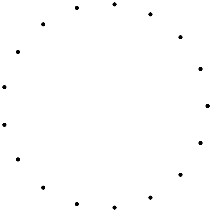
In our unified view, the domain of the uDTFT is the unit circle shifted up one. The unified Discrete Fourier Transform would also be points equally distributed about the circle, but with the origin as the anchor point. That feels better!

The Inverse Fourier Transform

I have always found the inverse cDTFT to be puzzling, since it is an integral in \(\omega\):

\[{\cal X}_{\mathbb{R}}^{-1}{F}(t) = \frac{1}{2 \pi} \int_{-\pi}^{\pi} F(e^{i \omega}) e^{i \omega t} \; d \omega.\]

The view that the domain of the cDTFT is actaully just a circle helps this integral make more sense. Really, the integral is a contour integral around the unit circle. The reason this integral looks like a real integral is that the unit circle has been parameterized and this form is a result of that parameterization.

The Nyquist Frequency

If the sampling rate is given by \(v\), the so-called Nyquist frequency is given by \(v/2\). If a signal has all its frequencies below the Nyquist frequency, then the signal can be perfectly reconstructed from the cDTFT. What does this mean in our scenerio? If the sampling rate is \(v\) Hertz then then time scale is \(\frac{1}{v} \mathbb{Z}\) (and it means that the angular velocity is \(2 \pi v\)). Therefore the region that the uDTFT is defined over is a circle of radius \(v\) centered at \(v i\). Remember, we have the view that frequency \(\omega\) is mapped to a point \(\xi\) on this domain (one could write \(\xi(\omega)\) to emphasize that \(\xi\) is a function of \(\omega\)).

The Fourier Transform on this time scale is

\[{\cal F}_{\frac{1}{v} \mathbb{Z}}\{f\}(\xi) = \sum_{t=-\infty}^{\infty} f(t) \frac{1/v}{(1+i \xi/v)^{t+1}}.\]

The relationship between \(\xi\) and \(\omega\) on this time scale is

\[\xi(\omega) = \frac{v}{i} (e^{i \omega/v} -1),\]

which again, can be thought as taking the unit circle, shifting it left by one, rotating it \(\pi/2\) radians to the left, then scaling up by factor of \(v\).

Notice that this relationship between \(\xi\) and \(\omega\) is \(2 \pi v\) periodic. One would think this would mean that there would not be overlap and confusion unless the frequency exceeded \(2 \pi v.\) However, there are symmetries (time reversal and conjugation) which essentially induce this overlap early - when the frequency exceeds \(\pi v\).

What I mean by overlap and confusion is that all frequencies that map to the same value of \(\xi\) will contribute to the Fourier transform evaluated at \(\xi\). This is called aliasing.

Perhaps what I like about this viewpoint is that there are two frequencies at work here. There is the sampling rate, which determines the size of the circle (the radius), and the variable frequency \(\omega\) which determines the angle from the cetner of the circle. So, the two frequencies act as the two components of a polar representation of the domain.

On a general time scale, there are many more frequencies at work (the time between samples is a function of time. But, this seperation is still at play. The sampling frequencies determine the shape of the domain (they won’t be circles anymore!) and the variable frequency \(\omega\) determines the location on the domain.

Two time steps.

Suppose that we have a signal that is sampled non-uniformly in time. For the sake of this example, let’s say the signal is sampled with a one-second gap, then a two-second gap, then a one-second gap, then a two-second gap, and so on. The sampling times form a time scale \(\mathbb{T}_{1,2} = \{\ldots, -7,-6,-4,-3,-1,0,1,3,4,6,7,ldots}.\) The unified Fourier Transform my colleagues and I have developed becomes, in this instance

\[\begin{aligned} {\cal F}_{\mathbb{T}_{1,2}}\{f\}(\xi) & = \ldots f(-7) (1+i \xi)^2 (1+2 i \xi)^2 + 2 f(-6) (1+i \xi)^2 (1+ 2 i \xi) \\ & + f(-4) (1+i \xi) (1+2 i \xi) + 2 f(-3) (1+i \xi) \\ & + f(-1) + \frac{f(0)}{(1+ i \xi)} + 2 \frac{f(1)}{(1+i \xi)(1+2 i \xi)} \\ & + \frac{f(3)}{(1+i \xi)^2 (1+2 i \xi)} + 2 \frac{f(4)}{(1+i \xi)^2 (1+2 i \xi)^2} + \ldots \end{aligned}\]

In order for the kernel to be bounded as \(t \rightarrow \pm \infty,\) it is neccesary and sufficient that

\[|(1+i \xi)(1 + 2 i \xi)| = 1.\]

The set of \(\xi \in \mathbb{C}\) for which this is true is shown below. This is the domain of this Fourier Transform. Note that the region is still tangent to the real axis and entirely in the upper-half plane.

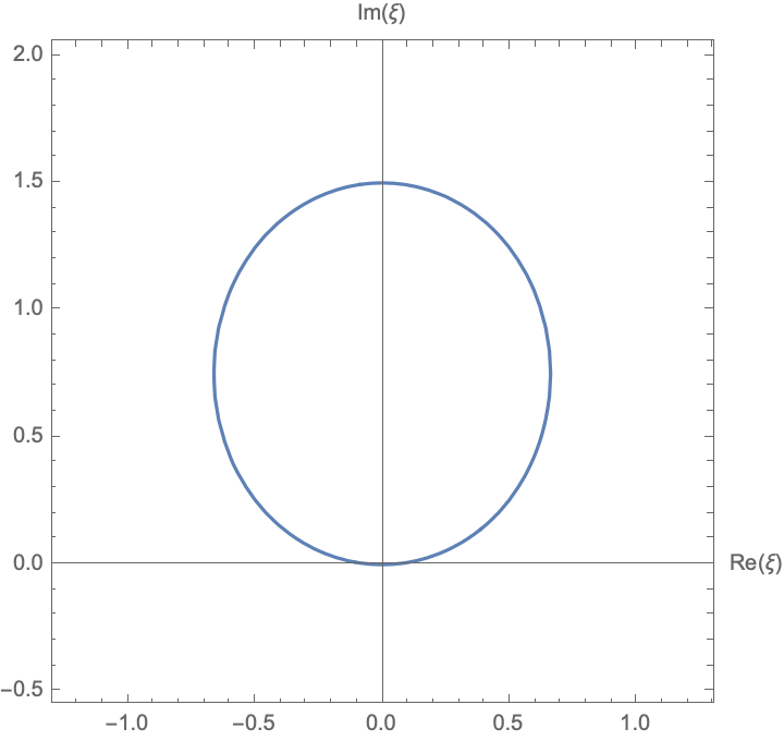
This region is in some sense the average of the unit circle tangent to the real-axis and the circle of radius 1/2 tangent to the real axis - ie/ the average of the domain of the Fourier Transform on \(\mathbb{Z}\) and the Fourier Transform on \(2 \mathbb{Z}\).

The mapping from frequency \(\omega\) to point in the complex plane \(\xi\) is complicated, even in this basic case. While the domain looks elliptical, it is not an ellipse. This mapping is, however, periodic with period \(4 \pi/3.\) This is again in agreement with the Nyquist frequency, as it has been proven that a signal can be reconstructed if the average sampling rate satisfies the Nyquist criterion and the signal has a finite bandwidth. Here, the average is two samples in three seconds, so \(v = 2/3\), and the Nyquist frequency should be \(2 \pi/3\), which is exactly half the peiod yet again!

Antarctic Ice Sheet Example

Consider the Vostok Ice Core CO2 Data, which shows CO2 concentrations over the past 419,000 years, sampled non-uniformly in time via an ice core sample. This gives us a signal \(f(t)\), where \(f\) is CO2 concentration, and \(t\) is defined on the time scale \(\mathbb{T} = \{-413649, -411959, -410653, -407331, -405523, -405523,\ldots\}\), measured in years, with \(t=0\) being the age of the ice at the last data point, 5679 years ago.

The time between samples is 1142.68 years on average, so we do expect the region where the Fourier Transform is defined to be relatively smaller than the regions we have encountered so far.

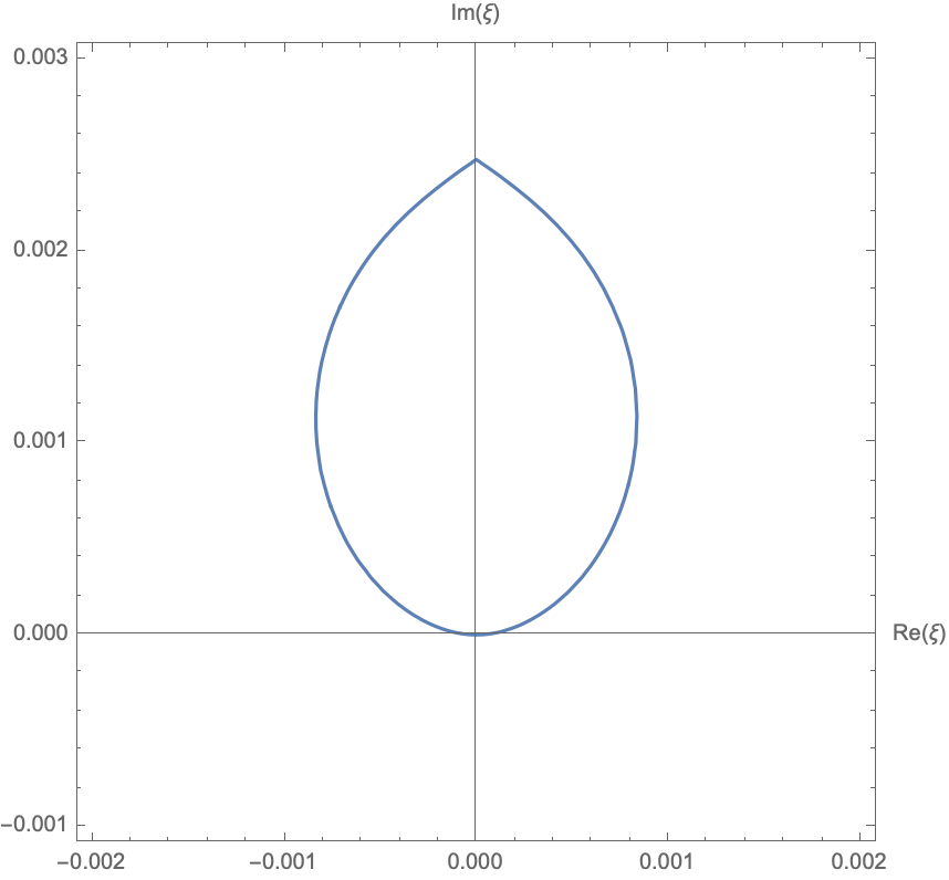Region where the Fourier Transform is defined for the Vostok Ice Core CO2 Data. It is almost lemon-shaped.

Again, we see that the sampling rate determine the domain of the Fourier Transform.

Below is the plot of the the signal versus time in years.

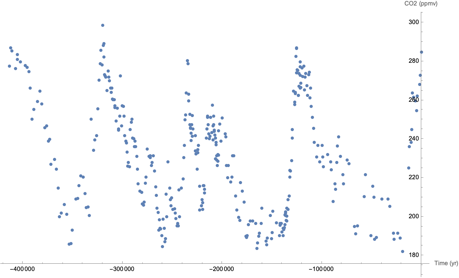
Just as with the Discrete Fourier Transform, in order to work with this signal effectively, we need to assume the signal is periodic. Moreover, our work assumes that the time domain is symmetric about the origin. Moreover, what is the time step between the last data point and the copy of the first data point when the signal repeats? We propose using the average time step in the signal, so as to not change the average and hence to not change the Nyquist frequency. Now the graph of the signal looks like the graph below, and continuing on in either direction to infinity.

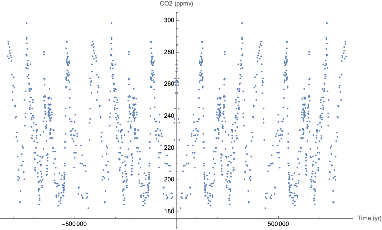
We are not saying that we know the CO2 levels 800,000 years into the future, we are just augmenting the signal to allow the theory to analyze the signal.

The Nyquist frequency for this example is \(\pi/1142.68\) radians per year, which corresponds to a period of 363.7 years. We should be able to detect patterns at this time scale and larger in the data.

Takeaways

• When considering Fourier Transforms, there are two frequencies that play a role. The sampling rate and the target signal frequency (the variable \(\omega\) in the cCTFT).

• The sampling rate of a signal manifests in the shape of the domain of the Fourier Transform.

• The domain of the Fourier Transform is parameterized by the target signal frequency \(\omega.\) The Nyquist frequency manifests in the periodicity of this parameterization.

• The cCTFT and cDTFT are really two manifestations of the same process. A simple change of variables helps us to see how the cDTFT becomes the cCTFT as the sampling rate goes to infinity.