Note: This blog post originally appeared on my Medium blog. I am reproducing the article here.

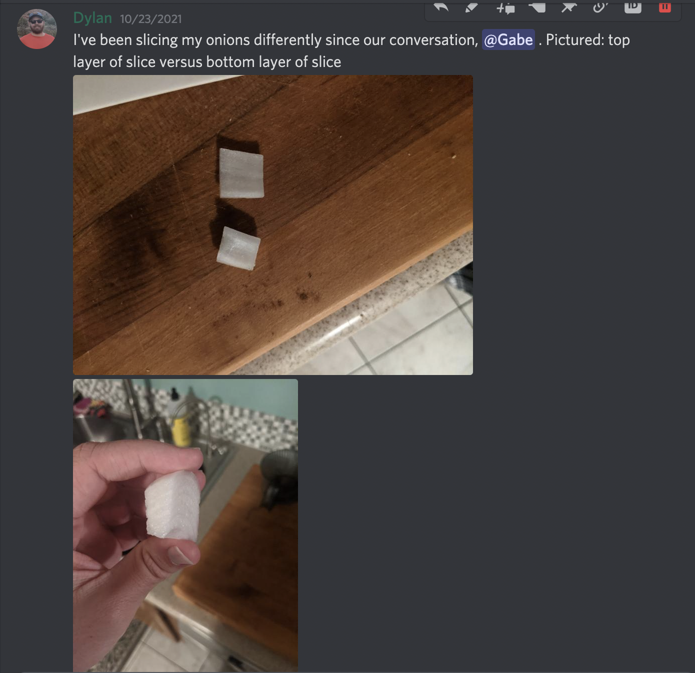
I first became interested in the the problem of cutting onions in a way to reduce the variance of the volumes of the slices at a gathering with friends. One of my friends and colleagues, Dr. Gabe Feinberg, also a mathematician, pointed me to the Youtube video below.

In the video, Chef Kenji López-Alt says he has a friend who is a mathematician, who claims that you should cut radially towards a point 60% of the radius below the center of the onion, and mentions that this might be related to the reciprocal of golden ratio, \(1/\phi = 0.61803398875...\)

I was intrigued by this, and even began cutting onions at home with this technique, just because it made me happy.

Each time I cut an onion for dinner, my mind would wander. I would think about why this is true, and what techniques I could use to approach the problem. While this was meditative for me, these musings did not lead anywhere substantial over the span of two months.

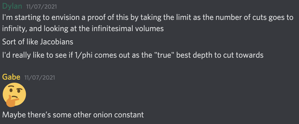
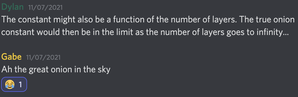
Last weekend, my thoughts actually lead me towards a solution. Within two days I had found the “true onion constant”, which, spoiler alert, is not the reciprocal of the golden ratio. The depth to which you have to aim your knife for radial cuts depends on the number of layers. You can see this by thinking of how to cut an onion with one layer versus an onion with ten layers to keep the pieces as similar as possible. For one layer you would aim towards the center of the onion, but for ten layers you would aim somewhere below the center of the onion. To simplify matters, I therefore thought of an onion with infinitely many layers (or, as Gabe called it, “the great onion in the sky,” which I love). These kind of abstractions are common in mathematics, and make problems tractable. Once there are infinitely many layers, it makes sense to think of infinitely many cuts. This moves the problem into the realm of continuous mathematics, where calculus can be used to great effect.

Here’s the technical part of the post. You probably need to know multivariable calculus to follow from here. I’m going to switch to using “we” instead of “I” to match mathematical writing conventions, and to indicate that we (you, dear reader, and I) are walking down this mathematical path together.

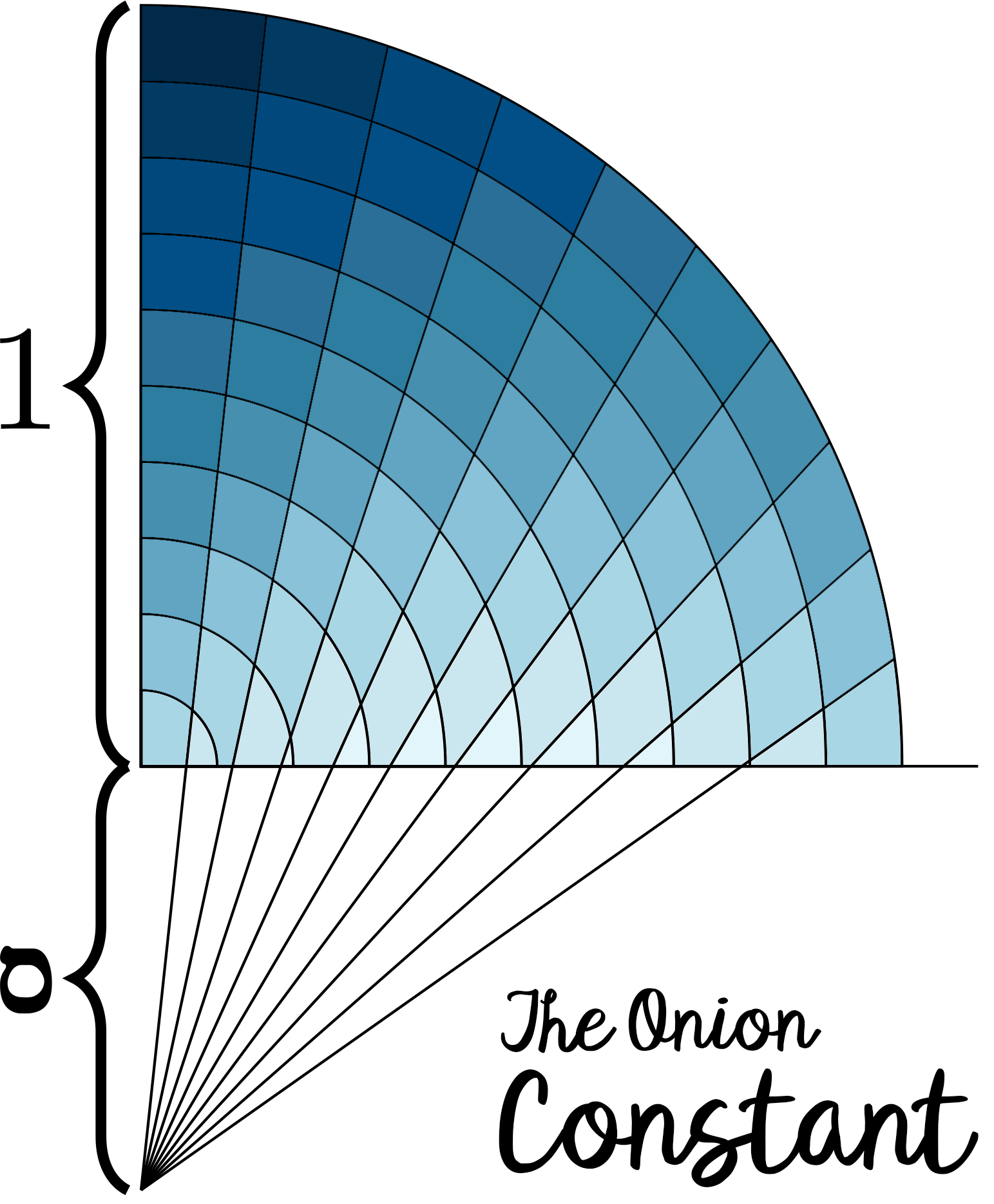
First, we model the onion as half of a disc of radius one, with its center at the origin and existing entirely in the first two quadrants in a rectangular (Cartesian) coordinate system. This ignores a dimension, and perhaps also some geometry of actual onions (are cross sections actually circles?) but makes the problem tractable and is still a good approximation.

The insight that leads to a solution comes from the Jacobian. When we change from rectangular coordinates to polar coordinates in integration, small rectangular pieces of area \(dx dy\) are transformed into small pieces of area \(r dr d \theta\), where \(x = r \cos(\theta)\) and \(y = r \sin(\theta)\). The idea of the Jacobian applies to all changes in coordinate systems. We can calculate the Jacobian as

\[J(r,\theta) = \frac{\partial x}{\partial r} \frac{\partial y}{\partial \theta} = r \cos^2(\theta) + r \sin^2(\theta) = r.\]

Below is a diagram showing the change of coordinates and the Jacobian in this setting.

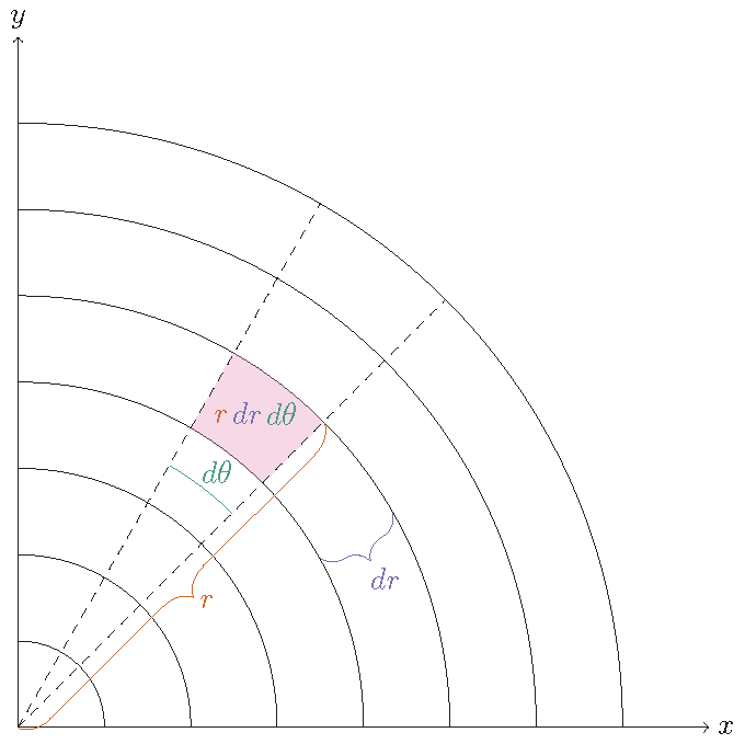
Notice that the coordinate system cuts the onion, much as usual grid lines cut the plane into rectangles in the Cartesian coordinate system. The radial part of the coordinate system cuts the onion radially (which of course nature does by default, but we need to model this mathematically), while the angular part of the coordinate system cuts the onion as our knife would if we were making straight cuts towards the center of the onion. Even though every piece of the onion is infinitely small (there are infinitely many layers, and infinitely many cuts) The Jacobian \(r dr d\theta\) gives a measure of how big the infinitely small pieces are relative to each other. Pieces near the center of the onion are smaller than pieces near the edge of the onion, as we can see that since \(r\) is smaller towards the center of the onion and larger towards the edge of the onion.

We can find the average value of the function \(f(r,\theta) = r\) over the part of the plane that defines the onion to find the average weight of the infinitesimal area, \(A\).

\[\overline{A} = \frac{\int_{0}^{\pi/2} \int_{0}^{1} r \; dr \; d \theta}{\int_{0}^{\pi/2} \int_{0}^{1} 1 \; dr \; d \theta} = \frac{1}{2}\]

Once we have the average, we can find the variance, \(\sigma^2\), of the weight of the infinitesimal area by calculating

\[\sigma^2 = \frac{\int_{0}^{\pi/2} \int_{0}^{1} (r-\overline{A})^2 \; dr \; d \theta}{\int_{0}^{\pi/2} \int_{0}^{1} 1 \; dr \; d \theta} = \frac{\int_{0}^{\pi/2} \int_{0}^{1} (r-1/2)^2 \; dr \; d \theta}{\int_{0}^{\pi/2} \int_{0}^{1} 1 \; dr \; d \theta}=\frac{1}{12}\]

The variance is a good measure of the uniformity of the pieces. If the variance is large, the pieces are not very uniform, and vice-versa.

The problem with this analysis, of course, is that we are cutting towards the center of the onion. We want to cut towards a point below the center of the onion. To accomplish this, we need a new coordinate system.

We make a coordinate system for cutting towards a point a distance \(h>0\) below the center of the onion. In this coordinate system, we measure the angle \(\theta\) from the point \((0,-h)\), while we measure the radius from the origin \((0,0)\) (both points in the rectangular coordinate system). The radial part of the coordinate system cuts the onion radially from the origin as before, while the angular part of the coordinate system cuts the onion as our knife would if we were making straight cuts towards the point \((0,-h)\), below the onion.

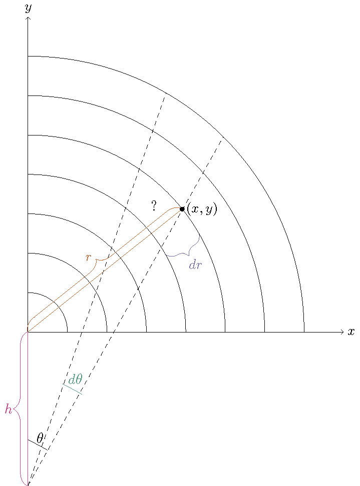
This coordinate system only works for the upper half plane, as there are now technically two points in the plane for a given point \((r,\theta)\). Luckily, our onion is entirely in the upper-half plane!

In this coordinate system, the region of the plane that we model as the onion is defined by \(0 \leq \theta \leq \arctan(1/h)\), and \(h \tan(\theta) \leq r \leq 1\). Notice that we are using symmetry. Usually we would think of the onion as a half-onion in the upper half of the plane. But, since the left side of the onion is a mirror image of the right side of the onion, and therefore both sides would have the same variance in area, we can perform this analysis just in the first quadrant.

The relation between \((x,y)\) and \((r,\theta)\) is less clear. Given we know \(r\), \(h\), and \(\theta\), we can draw the following triangle, with a new variable \(c\) which represents the distance from the point \((0,-h)\) to a given point \((x,y)\) (both in the rectangular coordinate system).

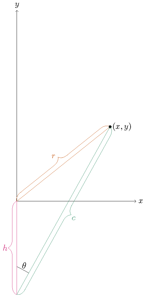
First, using the law of cosines, we can calculate

\[c=h \cos(\theta)+\sqrt{r^2-h^2\sin^2(\theta)}.\]

Using this, we can find the relationship between \((x,y)\) and \((r,\theta)\) as

\[\begin{aligned} x & = c \sin(\theta) \\ y & = c \cos(\theta)-h \end{aligned}\]

From this, for a given depth \(h\), we can calculate the Jacobian as

\[\begin{aligned} \scriptscriptstyle J(r,\theta) =& \scriptscriptstyle \frac{r \cos (\theta ) \left(\sin (\theta ) \left(-\frac{h^2 \sin (\theta ) \cos (\theta )}{\sqrt{r^2-h^2 \sin ^2(\theta )}}-h \sin (\theta )\right)+\cos (\theta ) \left(\sqrt{r^2-h^2 \sin ^2(\theta )}+h \cos (\theta )\right)\right)}{\sqrt{r^2-h^2 \sin ^2(\theta )}}\\ & \scriptscriptstyle -\frac{r \sin (\theta ) \left(\cos (\theta ) \left(-\frac{h^2 \sin (\theta ) \cos (\theta )}{\sqrt{r^2-h^2 \sin ^2(\theta )}}-h \sin (\theta )\right)-\sin (\theta ) \left(\sqrt{r^2-h^2 \sin ^2(\theta )}+h \cos (\theta )\right)\right)}{\sqrt{r^2-h^2 \sin ^2(\theta )}}. \end{aligned}\]

This is, to put it mildly, complicated. Nevertheless, we have done fairly straightforward calculus computations to get here, which shows the power of making this problem continuous. Mimicking what we did before, given a depth \(h\), we can find the average weight of the infinitesimal area, \(A(h)\), by calculating the integral of the Jacobian over the onion region divided by the integral of 1 over the same region

\[\begin{aligned} \overline{A}(h) &= \frac{\int_{0}^{\arctan(1/h)} \int_{h \tan(\theta)}^{1} J(r,\theta) \; dr \; d\theta}{\int_{0}^{\arctan(1/h)} \int_{h \tan(\theta)}^{1} 1 \; dr \; d \theta}. \end{aligned}\]

And the variance of the weight of the infinitesimal area, \(\sigma^2(h)\), is found by calculating the integral of the square of the Jacobian minus \(A(h)\) over the onion region divided by the integral of 1 over the same region

\[\sigma^2(h) = \frac{\int_{0}^{\arctan(1/h)} \int_{h \tan(\theta)}^{1} (J(r,\theta)-\overline{A}(h))^2 \; dr \; d\theta}{\int_{0}^{\arctan(1/h)} \int_{h \tan(\theta)}^{1} \; dr \; d \theta}.\]

Yikes! Integrating this by hand looks really difficult, if not impossible. We should use a computer to help us. Using the power of numerical integration in Mathematica, we can plot the variance versus h, the depth of the point we are cutting towards.

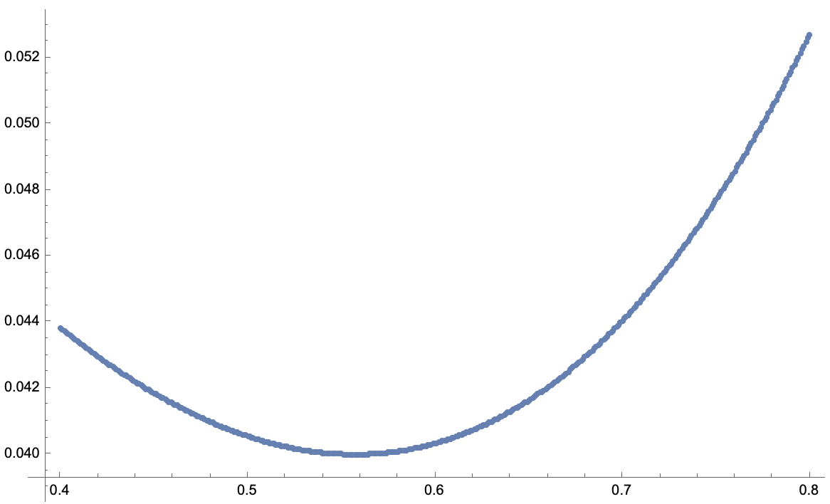
We can see the minimum variance is around \(h=.55\). We can use a numerical minimization technique to find the \(h\) that minimizes the variance.

I am only confident of this number to 7 decimal points, but the “true onion constant” for the “onion in the sky” is given by 0.5573066…

To get the most even cuts of an onion by making radial cuts, one should aim towards a point 55.73066% the radius of the onion below the center. This is close, but different from, the 61.803% suggested in the Youtube video at the top. Also, this number will be different for onions for finitely many layers (that is to say, all onions). Nevertheless, I find this answer to be beautiful, and I will forever treasure the true onion constant.

I think it would be interesting to consider the effect of the number of layers on this answer. Since with one layer the best strategy is to cut towards the center, I suspect that the best depth \(h\) to cut towards increases from zero with one layer, with 0.5573066… as the upper bound on the depth. So, the best depth for an onion with ten layers would be somewhere between 0 and 0.5573066. I have not investigated this in depth, but this seems like a fun next step.

I hope we all now know enough about onions to object.

Exo Comics 685

Update: I actually was able to evaluate \(\sigma^2(h)\) in a closed form. The techniques used to do it are really fun, and I am hoping to write them up for a recreational mathematics journal.

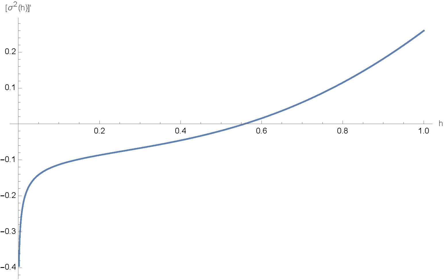
As calculus students know, if you want to minimize a function, you should take the derivative and set it equal to zero. Here, the derivative of \(\sigma^2(h)\) is given by

\[[\sigma^2(h)]' = \frac{k(h)}{48 \left(\cot ^{-1}(h)-\frac{1}{2} h \log \left(\frac{1}{h^2}+1\right)\right)^3},\]

where

\[\begin{aligned} &\scriptscriptstyle k(h)= \scriptscriptstyle -3 \pi ^2 \log \left(\frac{1}{h^2}+1\right) \\ & \scriptscriptstyle + 6 \left(h \log \left(\frac{1}{h^2}+1\right)-2 \cot ^{-1}(h)\right)^2 \left(h \left(h \log \left(4 h^2\right)+4 \sqrt{1-h^2} \left(\tan ^{-1}\left(\frac{h+1}{\sqrt{1-h^2}}\right)-\sin ^{-1}(h)\right)\right)+1\right)\\ & \scriptscriptstyle -2 \log \left(\frac{1}{h^2}+1\right) \left(h \log \left(\frac{1}{h^2}+1\right)-2 \cot ^{-1}(h)\right) \\ & \scriptscriptstyle \times \left(4 \left(1-h^2\right)^{3/2} \sin ^{-1}(h)-4 \left(1-h^2\right)^{3/2} \tan ^{-1}\left(\frac{h+1}{\sqrt{1-h^2}}\right)+h^3 \log \left(4 h^2\right)+h+2 \pi \right). \end{aligned}\]

The unique root of the above expression in the interval \((0,1)\) is the onion constant, since it is a critical point for the function \(\sigma^2(h)\) and the sign of \([\sigma^2(h)]'\) changes from negative to positive at this point, as seen in the graph of \([\sigma^2(h)]'\) below.

With this, I can calculate the onion constant to arbitrary precision. Here it is to 1000 decimal places:

0.55730669298566447885109305914592718083200030207273275933982921319 4698135127210458697529556348892779238421515729764144366026144985585 4165046873271472618959107816152780606384065758548635804885244580180 0007394442805906736214054844087432881741438971785006588976790490992 3546045053996637979358236569783223477190862479127621607686248472908 3731336235000704236891376747519710815301807822317779086701048122723 0239150930543232987021503400654503271867566236420521560986469125085 8159370220537524022076834487502663198536347064463252552885622069125 8227307037720900190873707797080215945078389222941122441664099620992 6654693052663485088353188368234518499463417515539540122160704233743 5539919306999218795184234750992607153483541905867849402571200687099 2663407278202945110198402208378584410140122892631419360798953694134 2227610384234804380488890547391245831871629728678785899984149264095 1979084439023291773013425234306472822863355983488650721455375797473 6357343027167265972675903577598983959532796594227162648681839040…

Such a beautiful mathematical constant deserves a name. I choose to use the Hebrew character samekh, because it looks particularly like an onion.