When I am not teaching or writing about mathematics, one of my hobbies is playing Pokemon games. In particular, I have been playing Pokemon Go for the past six years, and have recently started playing Pokemon Scarlet and Violet.

Pokemon Go has encouraged me to be active and to meet people both in my local community and around the world. I know people from my town that I wouldn’t otherwise know from the game. I have traveled to events and met people who I have befriended online. I find the games to be very relaxing, and a way to redirect my thoughts away from work.

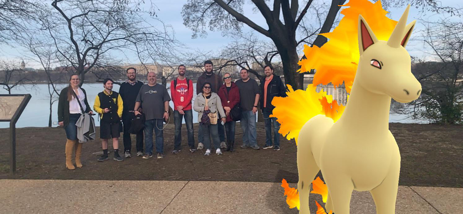A Group Photo at a meetup in Washington DC for members of a Discord server I administrate. I am third from the left.

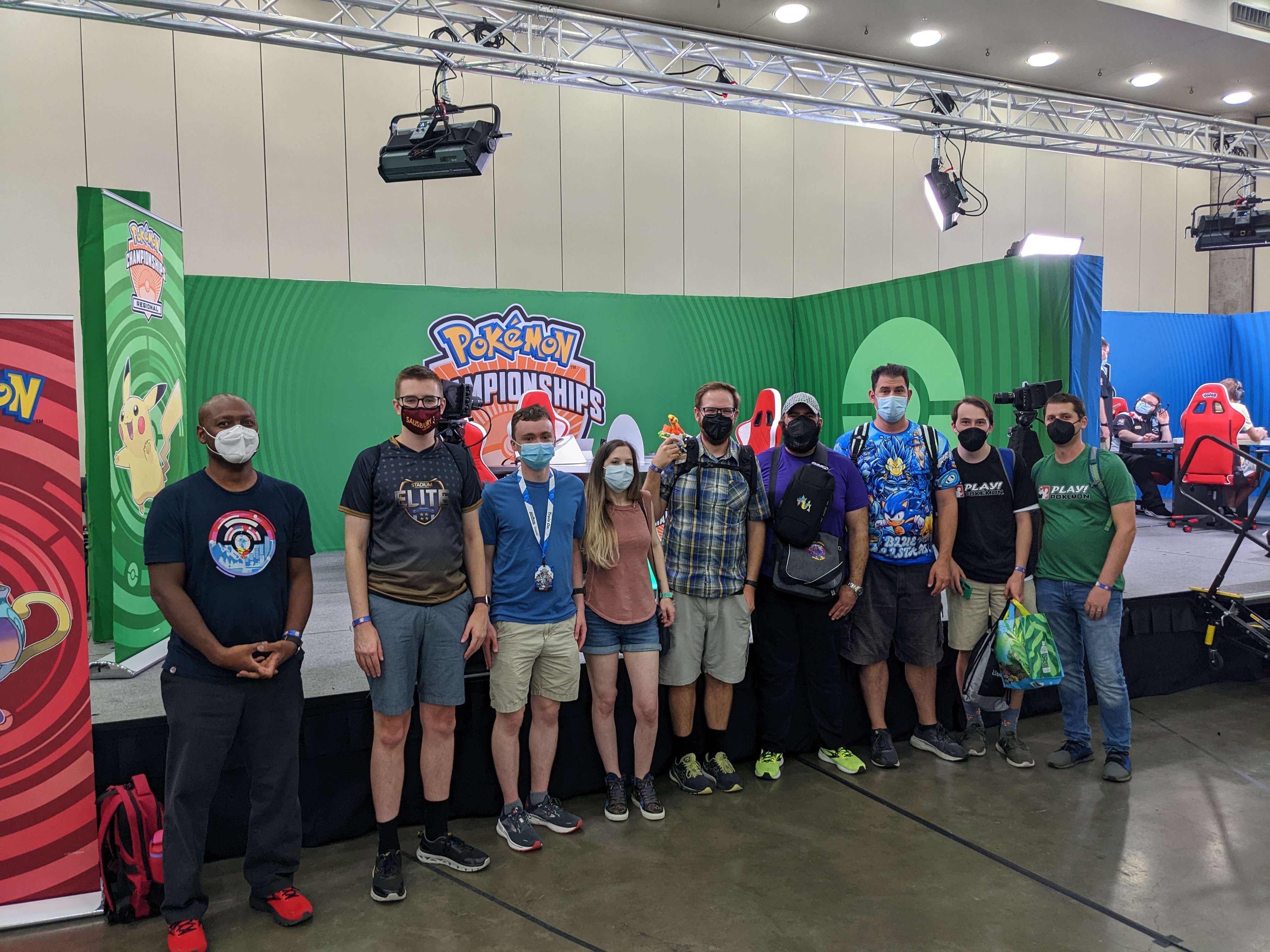A Group Photo at a Pokemon Go Tournament in Baltimore. I am in the middle in the yellow and blue shirt with the Ho-Oh on my shoulder. I know all these people from a Discord server that I administrate.

That said, I have a tendancy to look for the math in everything (although math is NOT everywhere, as I tell my History of Mathematics students). I have joked with colleagues that I could teach a whole introductory mathematics course on the math of Pokemon. One subject in that course would be probability theory via shiny hunting.

A shiny Pokemon is a differently-colored version of a Pokemon that appear randomly and very rarely. Although they are purely cosmetic, they are highly sought after trophies, with people dedicating hours, days, even months, trying to find a shiny Pokemon. So many Twitch and Youtube streams are dedicated to shiny hunting. So. Many.

Shiny Pokemon hunting is a wonderful lens through which to understand some of the most important concepts in probability theory: Independence, Bernoulli trials, the binomial distribution, the geometric distribution, the Poisson distribution, the exponential distribution, and the memoryless property. Let’s take each of these in turn.

Independence

In Pokemon Scarlet and Violet,the probability that an individual Pokemon will be shiny is 1/4096. With certain methods in the game, this probability can be increased up to 1/512. Whether a given Pokemon is shiny or not does not depend on whether another Pokemon is shiny or not. In probability, we say that shininess is independent of Pokemon.

When calculating the probability that two independent things happen, one simply multiplies the probability that the first thing happens by the probability that the second thing happpens. For example, the probability of 1) flipping a fair coin and getting a head and 2) rolling a five on a fair six-sided dice is \((1/2) (1/6) = 1/12\).

Bernoulli Trial

A Bernoulli trial is a fancy way of saying “flipping a weighted coin.” Technically, a Bernoulli trial is an experiment where “success” occurs with probability \(p\), and “failure” occurs with probability \(1-p\). There are no other options (here failure is an option).

Let’s recast this definition in terms of Pokemon. Checking whether one Pokemon is shiny (hereafter known as a shiny check) is a Bernoulli trial where “success” means the Pokemon is shiny, and “failure” means the Pokemon is not shiny. The value for \(p\) is \(1/4096\) (without any boosts).

Binomial Distribution

When hunting for shinies, people do not just check one Pokemon and call it a day. The name of the game is to check as many Pokemon as possible as quickly as possible. This means the Bernoulli trial is repeated, and each trial is independent. Let’s say a streamer was going to check 1000 Pokemon, then give up. They are curious in knowing the probability that they see zero shinies, one shiny, two shinies, and so on. The binomial distribution would sate their curiosity.

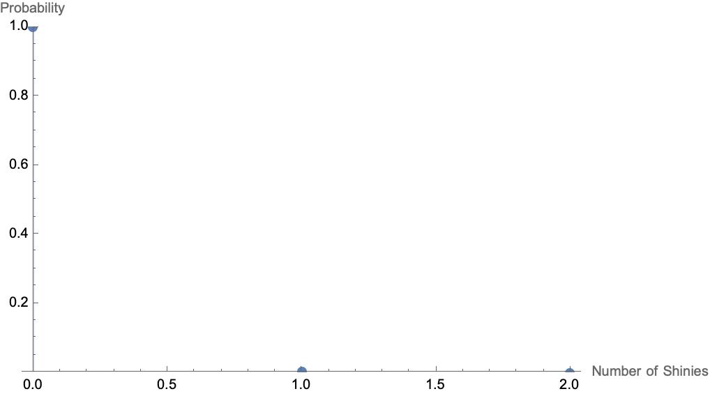
For \(p=4096\), the probability mass function of the binomial distribution is plotted below. On the \(x\)-axis is the number of shinies, and on the \(y\)-axis is the probability.

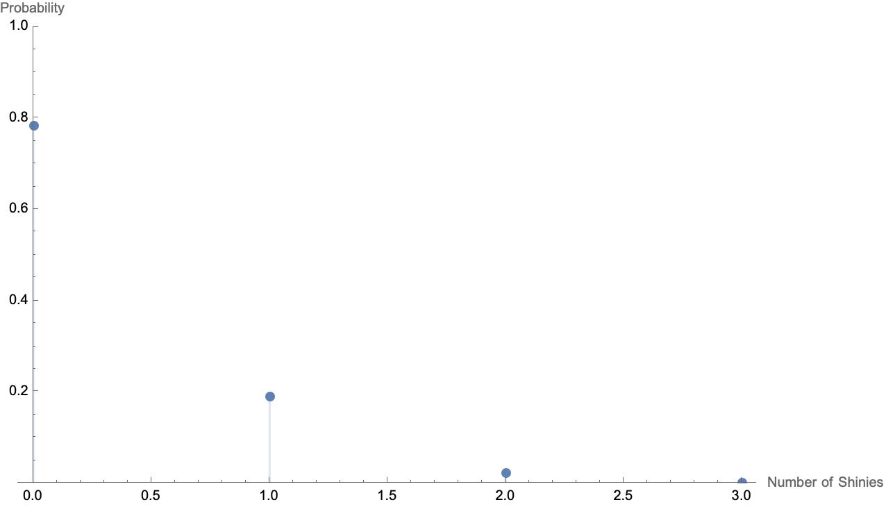
The probability that the streamer fails the entire shiny hunt is almost \(80\%\), while the probability of getting one shiny is almost \(20\%\). There is a small probability of getting two (or more!) shinies.

Let’s break down one of these probabilities. If the streamer were to get one shiny, then they would have 999 failures and one success. The probability of this is \((1/4096)^{1} (4095/4096)^{999}\). But, this does not account for the order that the streamer finds a shiny. They could find the shiny on the first check, or the second check, or the third check, and so on until the 1000th check, which means there are 1000 different orders. The probability of getting exactly one shiny in 1000 checks is then

\(1000 (1/4096)^{1} (4095/4096)^{999} \approx 0.191...,\) or, about 19.1%.

If the streamer were to use all the available methods (complete the Pokedex to get the shiny charm, go to a mass outbreak and clear sixty or more Pokemon, and make a level three sparkling power sandwich), and make \(p=1/512.44\) ¹ during the 1000 Pokemon hunt, the probability mass function for the binomial distribution would instead look like the graph below.

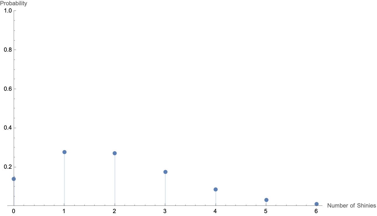
The probability of failing the hunt (getting zero shinies) has decreased from nearly \(80\%\) to about \(14\%\). There is also a much higher probability of two or more shinies during the hunt. The extra effort to increase \(p\) seems to be worth it.

Side Note About the 1/512.44 Probability

The way the boosts in shiny rate work is that instead of doing one Bernoulli trial with \(p=1/4096\) to determine shininess, the game does more than one Bernoulli trial to determine shininess (with the number of trials determined by the boost). If any of these trials are successful, then the Pokemon is shiny. A shiny charm changes the number of Bernoulli trials to three, while the 1/512.44 rate comes from the number changing to eight trials. Why? Let’s work it out!

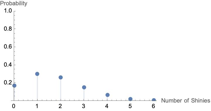
Let’s look at the binomial distribution with \(p=1/4096\) as before, but with \(8\) trials instead of \(1000\).

That looks like the probability of zero successes in eight rolls is one, but this is why graphs can be misleading. Let’s do the math.

The probability of zero successes in eight independent trials is (by the multiplication rule) \((4095/4096)^8 \approx 0.99804954\). So the probability of more than one success (and therefore of a shiny Pokemon being produced) is about \(p_{\text{shiny}} = 1-.99804954 \approx 0.00195146\). Converting this to a fraction with one in the numerator gives \(1/512.4376602...\), which the Bulbapedia ¹ rounds to \(1/512.44\).

The Geometric Distribution

Oftentimes, a shiny hunter will not be interested in multiple shinies of the same Pokemon. They will stop the hunt if and only if they find one shiny. Here, the shiny hunter is not interested in the number of shinies they get for a fixed number of checks, but instead is interested in the amount of checks until a shiny is found. The geometric distribution addresses this idea.

The geometric distribution gives the probability of number of Bernoulli trials until the first success for each possible number of trials. If a person is full-odds shiny hunting (\(p=1/4096\)), the geometric distribution for the number of checks until a shiny is found is shown below.

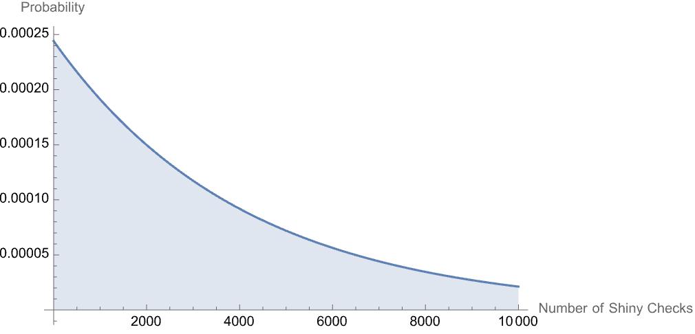
First, notice how the \(x\)-axis is now “Number of Shiny Checks.” Also, The probability axis has very small numbers. This is because the probability (which adds to one) is spread out over many, many possibilities. In this context, it doesn’t make much sense to talk about the probability of it taking exactly, say, 4000 checks to get a shiny. Instead, it is more informative to to look at the probability that it take less than, say, 4000 checks to get the shiny. This idea is called the cumulative distribution function. For a geometric distribution with \(p=1/4096\), the cumulative distribution function has the graph plotted below.

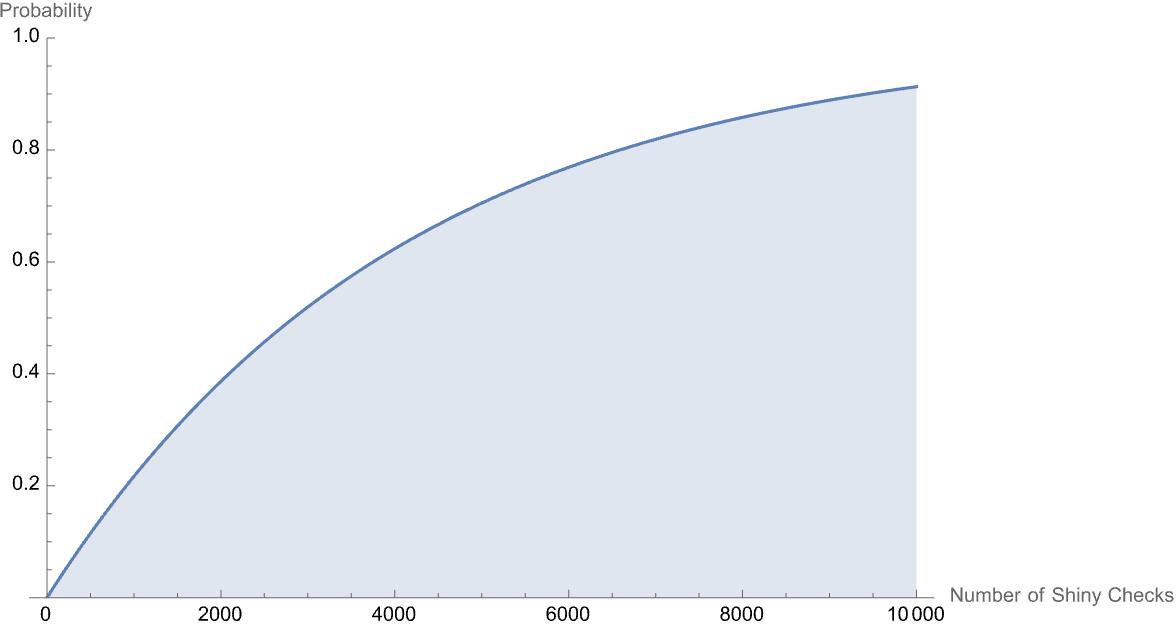
Some features I notice really quickly:

1) If a shiny hunter does 4096 checks, the shiny is not guaranteed. In fact, there is only about a 63% ² chance that the shiny will appear in the first 4096 checks. Even worse, as the number of checks gets large, the function levels off but never actually equals one. This means a shiny is never guaranteed.

2) It takes about 2838 checks in order for there to be a 50% chance of getting a shiny. I think most people would guess 2048 checks.

Some other features are less apparent. One of my favorite facts is that if someone has already checked some shinies, the cumulative distribution function for how many more checks until they encounter a shiny has exactly the graph above. This is called the memoryless property. This should feel both obvious and strange. I like to think about coin flipping. If I flip five heads in a row, but I know the coin is fair, the probability that the next coin is heads has not changed from \(1/2\). The past results have no impact on the future in this regard. So, if someone has already checked 10,000 Pokemon for shininess and has come up empty-handed, the probability that they’ll find a shiny in the next 4096 checks is still only 63%. There’s no credit earned from the universe from those first 10,000 checks.

The Poisson Distribution

In Pokemon, the shiny checks, which are discrete events, still happen in continuous time. Instead of thinking about the number of shinies in a certain amount of checks, as in the Binomial Distribution, one could instead consider the number of shinies in a certain amount of time.

Let’s work with an example. Yesterday, while home sick, I set aside 30 minutes to shiny hunt Magnemite in a mass outbreak with \(p=1/512.44\). Using a technique known as “picnic resetting” I was able to shiny check 15 Magnemite in, on average, 30 seconds (yes, I kept track). This means in 30 minutes, I would do approximately 900 checks. If I had hours and hours to play, I might expect that I would get \(900/512.44 \approx 1.756\) shinies per 30 minute period. But, due to randomness, the amount I get in just one 30 minute period might be larger or smaller. The amount of shinies I get in a 30 minute period with an average amount of 1.756 can be modeled by a Poisson Distribution, a distribution that models the number of rare events that occur in a unit of time.

The probability mass function for the Poisson distribution with an average value of 1.756 is shown below.

We can compare this to a Binomial distribution with \(p=1/512.44\) over 900 shiny checks.

They look very similar, and this is hopefully not a surprise (they are modeling the same thing, after all)! This is a wonderful illustration of the Poisson Paradigm, which states that the Poisson Distribution and the Binomial Distribution are very similar when the probability of success is small and the number of trials is large. One advantage in using the Poisson distribution is that the probabilities are easier to calculate. Another advantage is that we have shifted our thinking from discrete events that exist outside of time thinking of these checks as existing in time.

The Exponential Distribution

The geometric distribution models the amount of shiny checks until the first success. Given the shift to continuous time in the Poisson Distribution, it makes sense to think about the amount of time until the first shiny appears. A big shift has occured here, since time is continuous, not discrete like the previous distributions. The name of the distribution that models the time between rare events with a given average number of events is the exponential distribution.

Continuing with the example in the previous section, I ask how long should it take to find a shiny Magnemite in a mass outbreak (remember that I only have 30 minutes)? I need a average, which I know is 1.756 per 30 minutes. But, if I want a plot where the \(x\)-axis is time in minutes, I should adjust this average to be 1.756/30 per minute. Below is the cumulative distribution function for an exponential distribution with average 1.756/30 versus time in minutes.

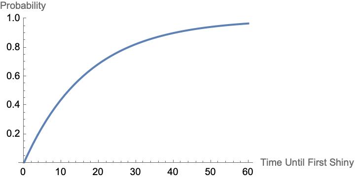
According to this model, there is about an 82% chance that I will find the shiny in the thirty minutes I set aside for shiny hunting. If I give myself an hour, the probability increases to 97%. But, cruelly, if I don’t find one in the first 30 minutes, the probability that I find one in the next thirty minutes is only 82%, not 97%. Again, the universe doesn’t give credit for past effort in these regards. The memoryless property strikes again!

The Memoryless Property

Both the Geometric Distribution and the Exponential Distribution have the memoryless property. In fact, they are the only two distributions that have this property.

Conclusion

The Binomial Distribution and the Poisson Distribution are intricately linked, as are the Geometric Distribution and the Exponential Distribution. In fact, I wrote an academic paper that makes this link explicit, showing that they are the result of the same process on different time domains. ³

Even the silly and recreational things in life can lead to interesting and deep ideas if pursued (that is perhaps the entire premise of this blog). That said, getting at deep and interesting ideas should not always be the goal in life. Sometimes, it’s just fun to kick back, relax, and look for differently colored digital monsters.